About Ebola Dataset

A sample dataset used in this Ebola Predictive Model covering parts of Guinea, Sierra Leone and Liberia in Africa consists of six layers; Districts, Airports, Community Care Center (CCC), Ebola Treatment Center/Units (ETC), Logistic Base (LBS) and Roads. Metadata including Geometric type and Coordinate Reference System (CRS) is summarized in Table 2. The geometric features of Ebola dataset displayed in Figure 7.

Layer	Use of geo-analysis	CRS	Type
districts	Guinea, Liberia, Sierra Leone	3857	Polygon
airports	Airports in the countries	3857	Point
ccc	Community Care Center	3857	Point
etc	Ebola Treatment Center and Units	3857	Point
lbs	logistic bases	3857	Point
Roads	Roads	3857	Line
Maplink	OpenStreetMap	3857	TMS

Table 2. Metadata of Ebola dataset

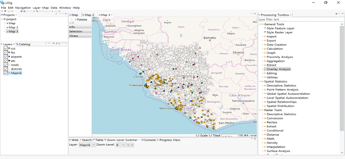Figure 7. Ebola Dataset displayed on uDig SW

Ebola Predictive Model

The Ebola Predictive Model in Figure 15 used in this paper was provided by the UN. Geospatial analysis functions of ArcGIS SW written in the Ebola Predictive Mode. Each function in the Ebola Predictive Model corresponds to a geospatial analysis function of Spiral 3. For instance, Select, Merge, Split, and Clip correspond to the same of geospatial analysis functions of Spiral 3. Some of these operations are integrated into one operation.

While Whereas analysis sequence of a road layer consists of three steps (Select Clip Line Density) in the Ebola Predictive Model in Figure 15, it consists of two steps (Point in Polygon Line Density) in Feature 8. It is because Line Density function of Spiral 3 automatically executes Clip operation as a parameter of Line Density. Since the result can be generated by executing a less number of geospatial analysis functions, it becomes an advantage of the Spiral 3 approach in terms of user convenience.
The Ebola Predictive Model is simplified as shown in Figure 8 by using geospatial analysis functions of Spiral 3. To execute the Ebola Predictive Model in Figure 8, Point in Polygon operation for vector dataset, Line Density and Zonal Statistics for raster dataset and Ordinary Least Squares Regression (OLS) for spatial statistics in Spiral 3 were applied.

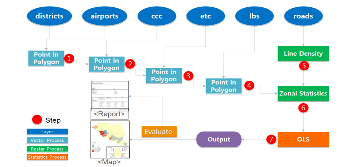Figure 8. Simplified Workflow of Ebola Predictive Model

Analytic Process

The first step of simplified Ebola Predictive Model in Figure 8 is Point in Polygon overly function. It creates a new district layer by adding a new column with a number of airports in each district.

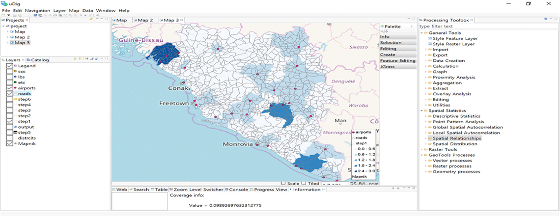Figure 9. Point in Polygon Result: districts

The processes from the second to the forth steps are the same as the first one except parameters. Once the fourth step is done, each district will have columns with each number of airports, LBSs, CCCs, and ETCs.
The fifth step is for the Line Density of Spiral 3. When the Line Density function is selected from the Processing Toolbox, which contains the geo-analysis functions of Spiral 3, it requests line feature as an input data, which is a road layer in this use case. The Line Density function automatically executes Clip operation by parameterizing. For instance, districts were set as an extent for clipping during the Line Density process in the Figure 10.

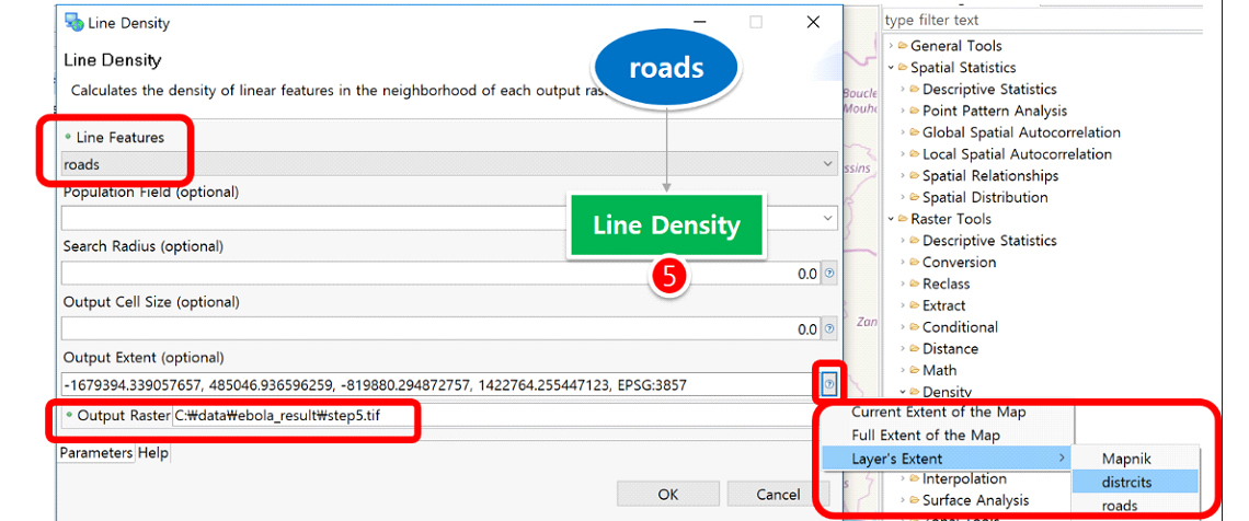Figure 10. Parameters for Line Density

The sixth step is Zonal Statistics. It calculates the road density of each district.

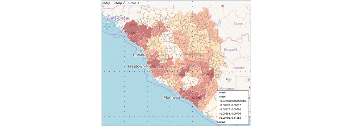
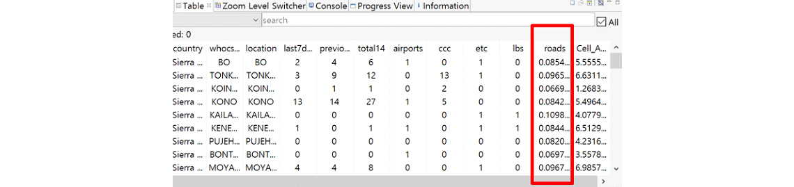Figure 11. Result of Zonal Statistics: districts with road density

The last step is Ordinary Least Squares (OLS) Linear Regression. The OLS calculates how the facilities such as airports, logistic bases (lbs), Ebola Treatment Centers (etc), community care centers (ccc), and roads affect Ebola occurrence. The facilities therefore become explanatory variables in the OLS step. Ebola occurrence is coded as a dependent variable tot14 in Figure 12.

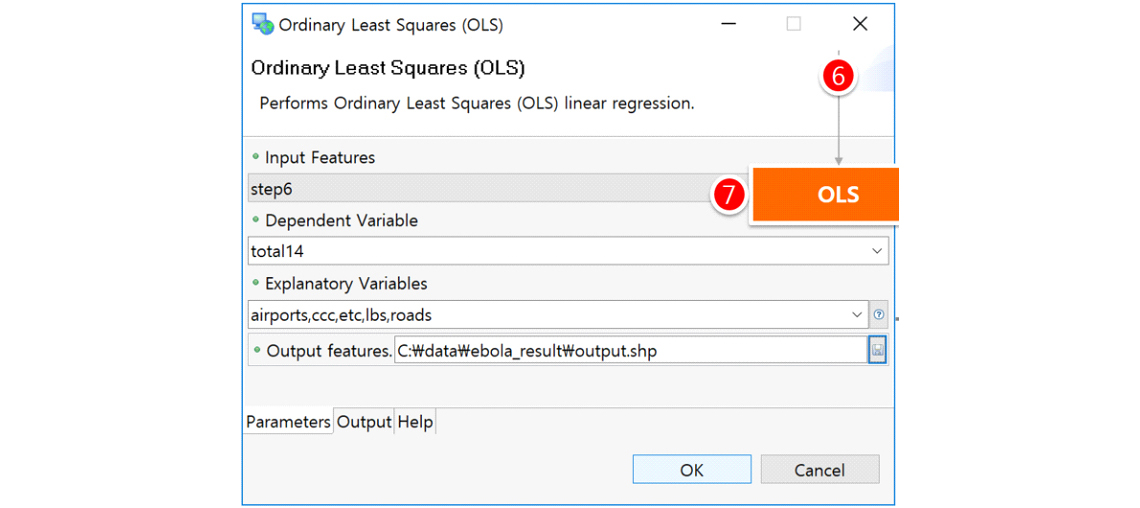Figure 12. Parameters for OLS 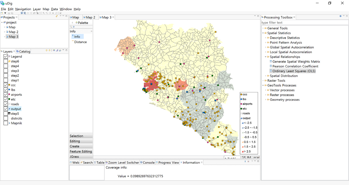Figure 13. Output of OLS: districts re-classified with residual standard deviation 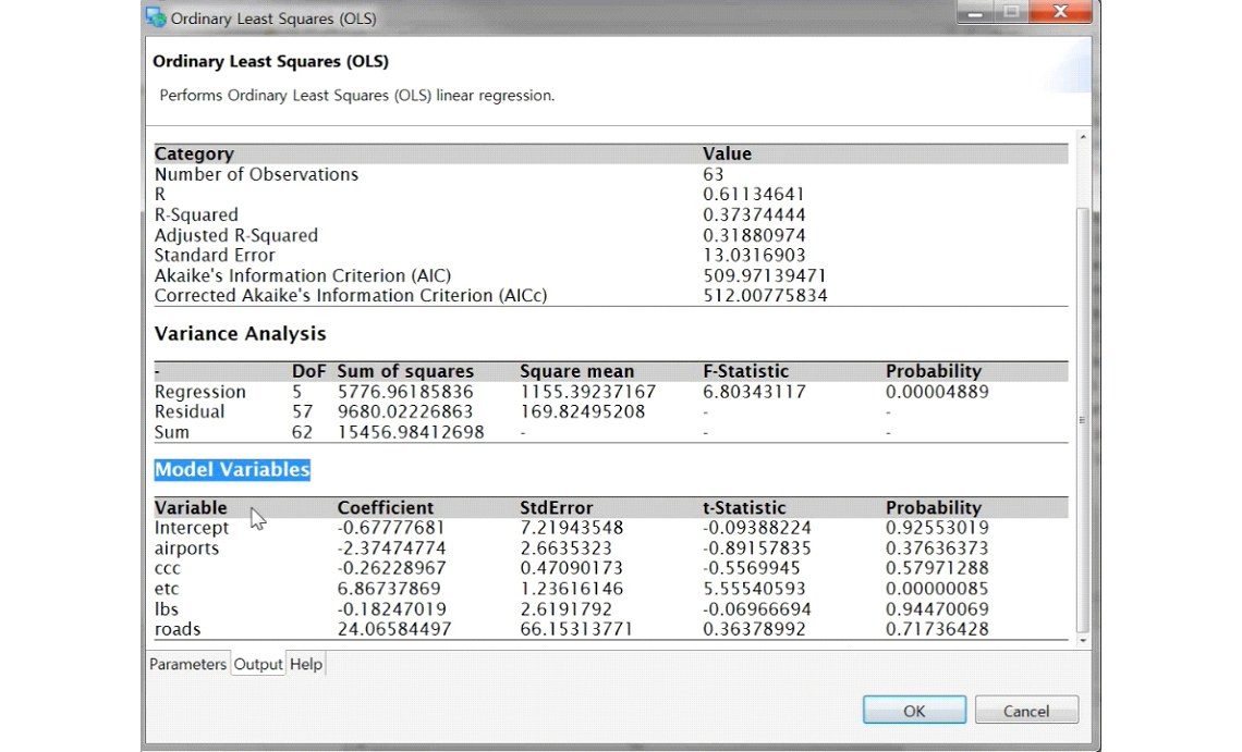Figure 14. Statistical Report of OLS

Lessons Learned from the Use-Case

From this use-case, we learned the following lessons. First, the clean data set is essential for accurate results of the analysis. Noisy and incorrect data not only degrade the accuracy of the results but also make the analysis process time consuming due to the data cleaning steps.
Second, user-friendly interface and functions facilitate the geo-analytical process. Considering most users of the geo-analytic tool are not GIS experts, user-friendly interfaces such as model builder make the tool more accessible to wider user group.
Third, we have to validate the result of our geo-analytic tool in comparison with proprietary commercial tool. During this use-case, we found that the results of some analysis by our tool slightly differ from those with a proprietary commercial tool. Unfortunately, the internal approach and methods used for geo-analytic functions in the proprietary commercial tool are not accessible.